Parameter Calculation

First I set Duty Cycle to be 80, and let the car run straight towards a wall and recorded the value of TOF. Then I use the data to calculate the speed of the car while also verifying the reliability via linear fitting.

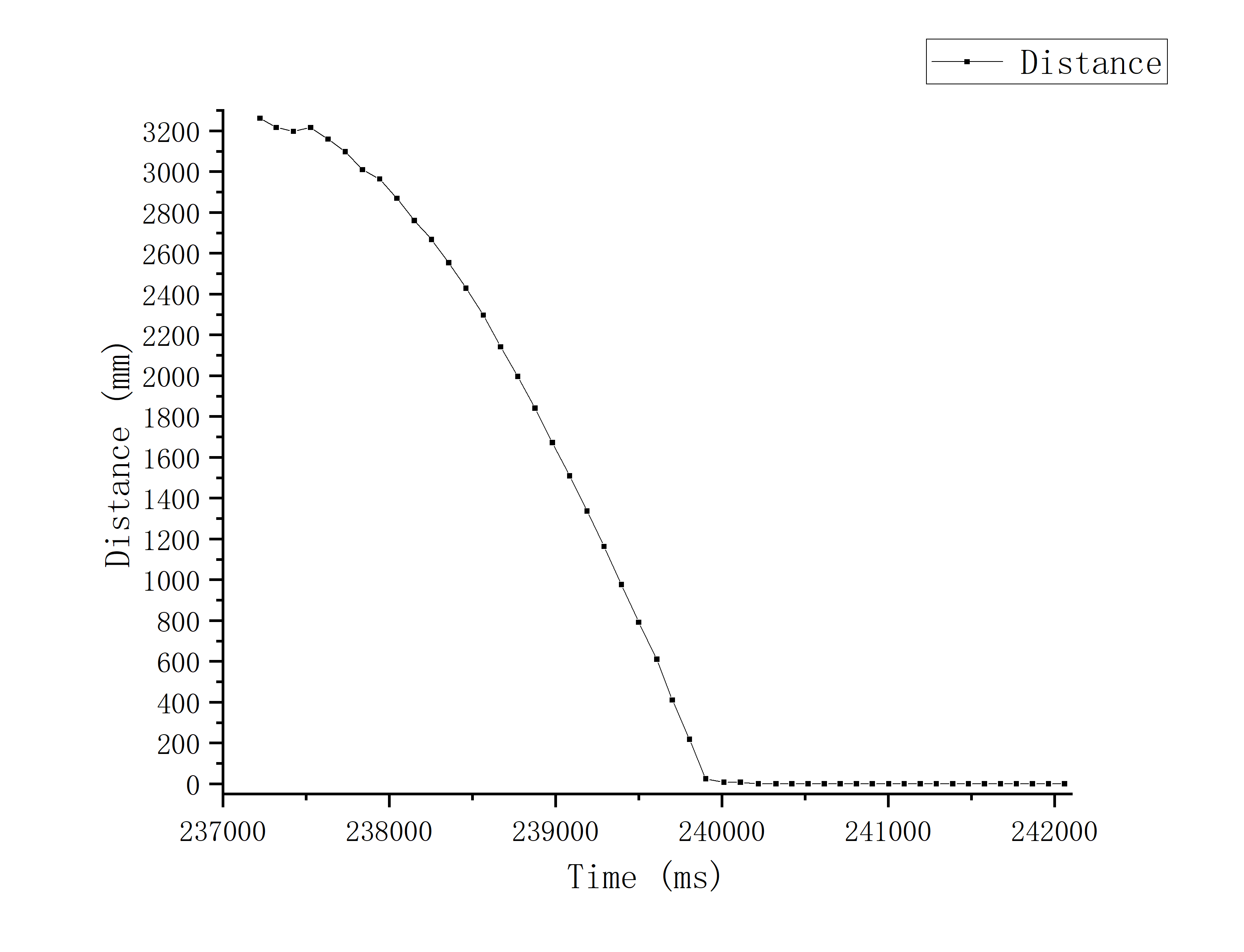
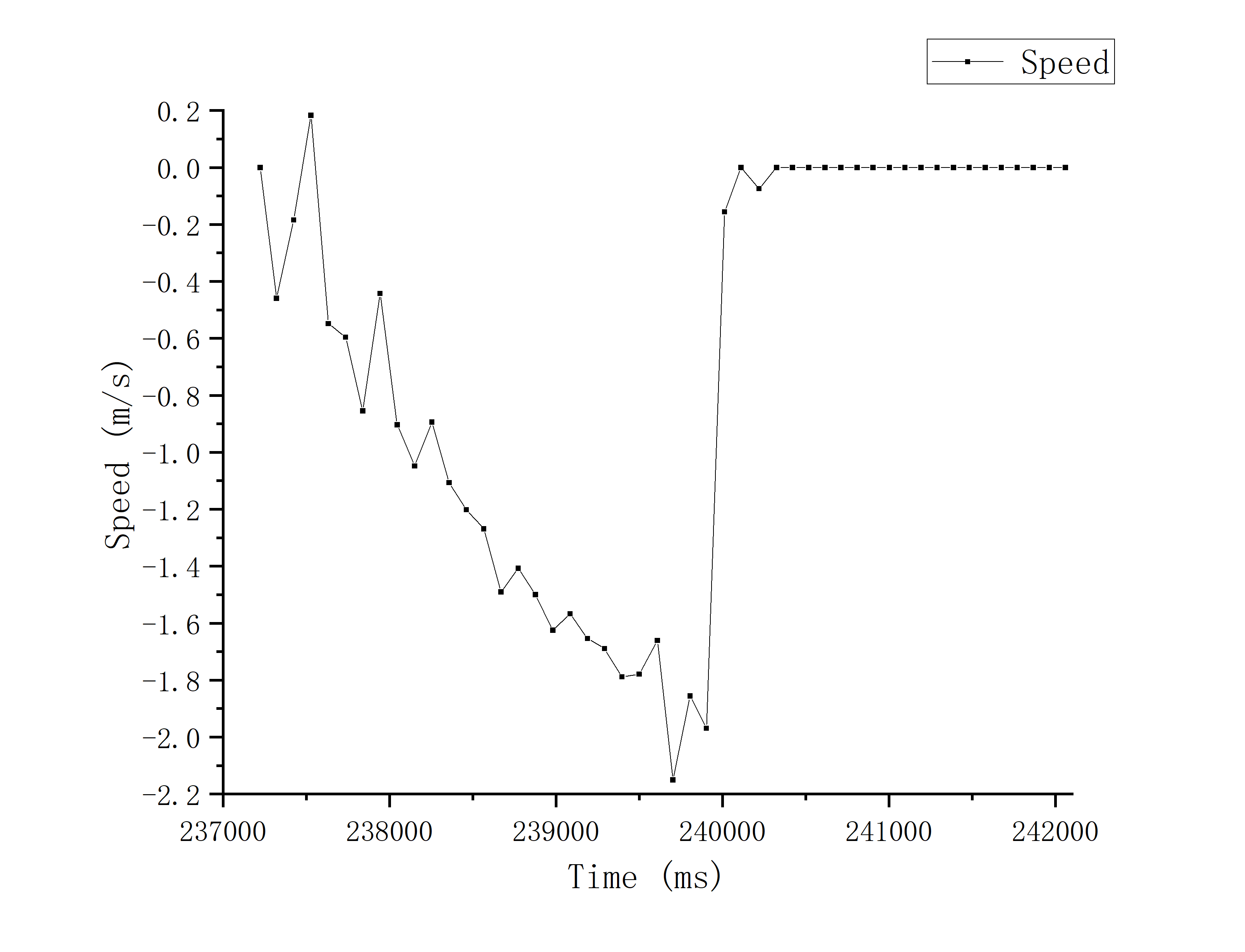
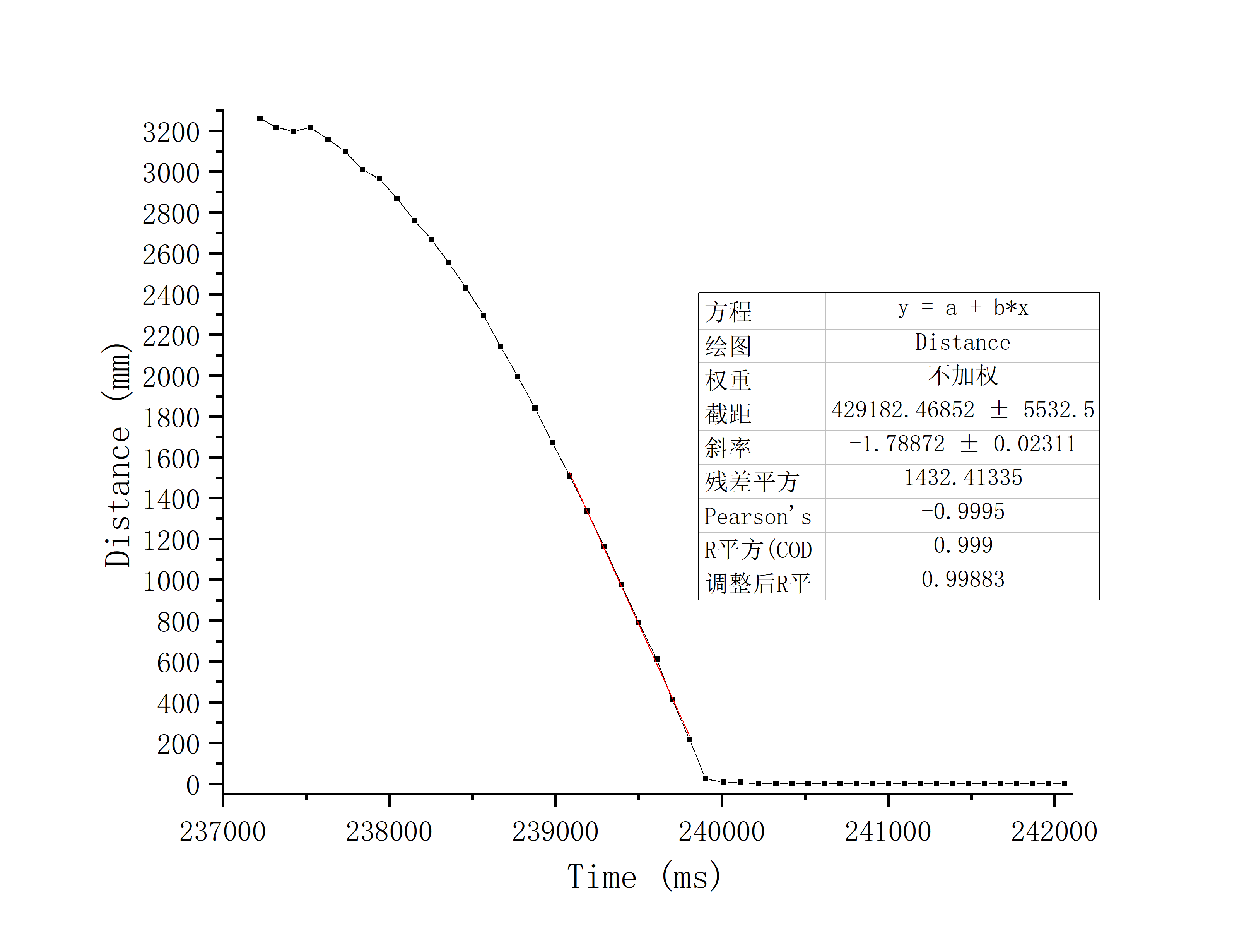
As can be seen from the above figures:
Starting time: 237.223ms
Time to reach maximum speed: 239.396ms
Maximum speed: ~1788.72mm/s

d = 80/1788.72 = 0.04472
For 'm', I first calculated the m value of each point, and then selected a point with a relatively stable value in the middle position for calculation:
m = -dt_0.67 / ln(1-0.67) = 0.04972
So the matrix A, B, C are showed below: (I change the C matrix from [-1 0] to [1 0] because the distance from the wall decreases as the car moves forward)

Kalman Filter Setup

I set both σ₁ and σ₂ to be √(10²·1/d_t), and σ₃ to be 20.
Then I have the Noise Matrix Σ_μ and Σ_z :

I use the data in Lab6 (including Time, Duty Cycle, Distance) to simulate the Kalman Filter in Jupyter Lab under the conditions of no update and update respectively:

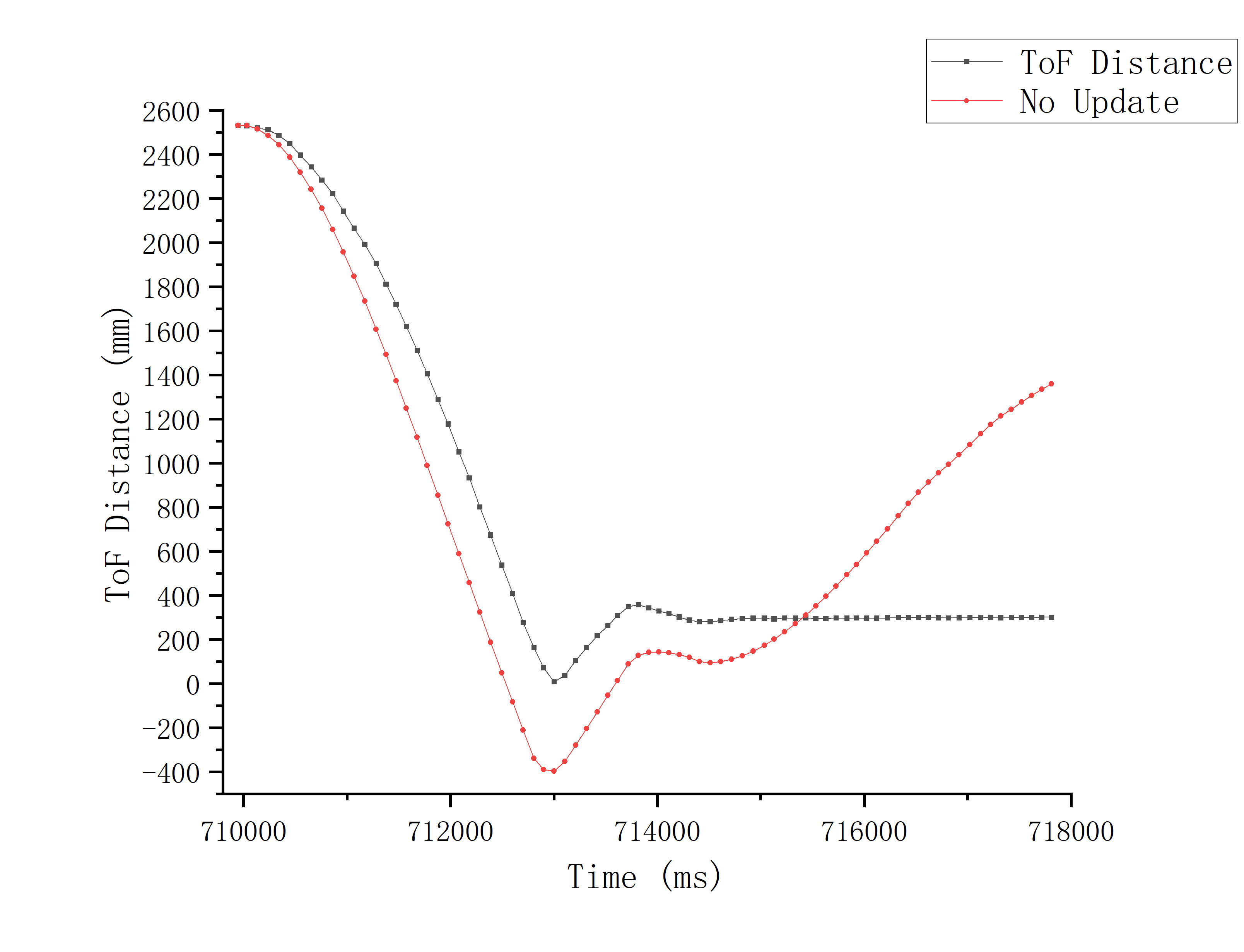
From the results above, it can be seen that the general trend of the simulation is consistent under the condition of only prediction. However, when the car adjusts its position back and forth near the set_point, a relatively large error occurs due to the rapid transition of duty cycle and the influence of ground friction, which leads the prediction curve to gradually deviate from the actual position.

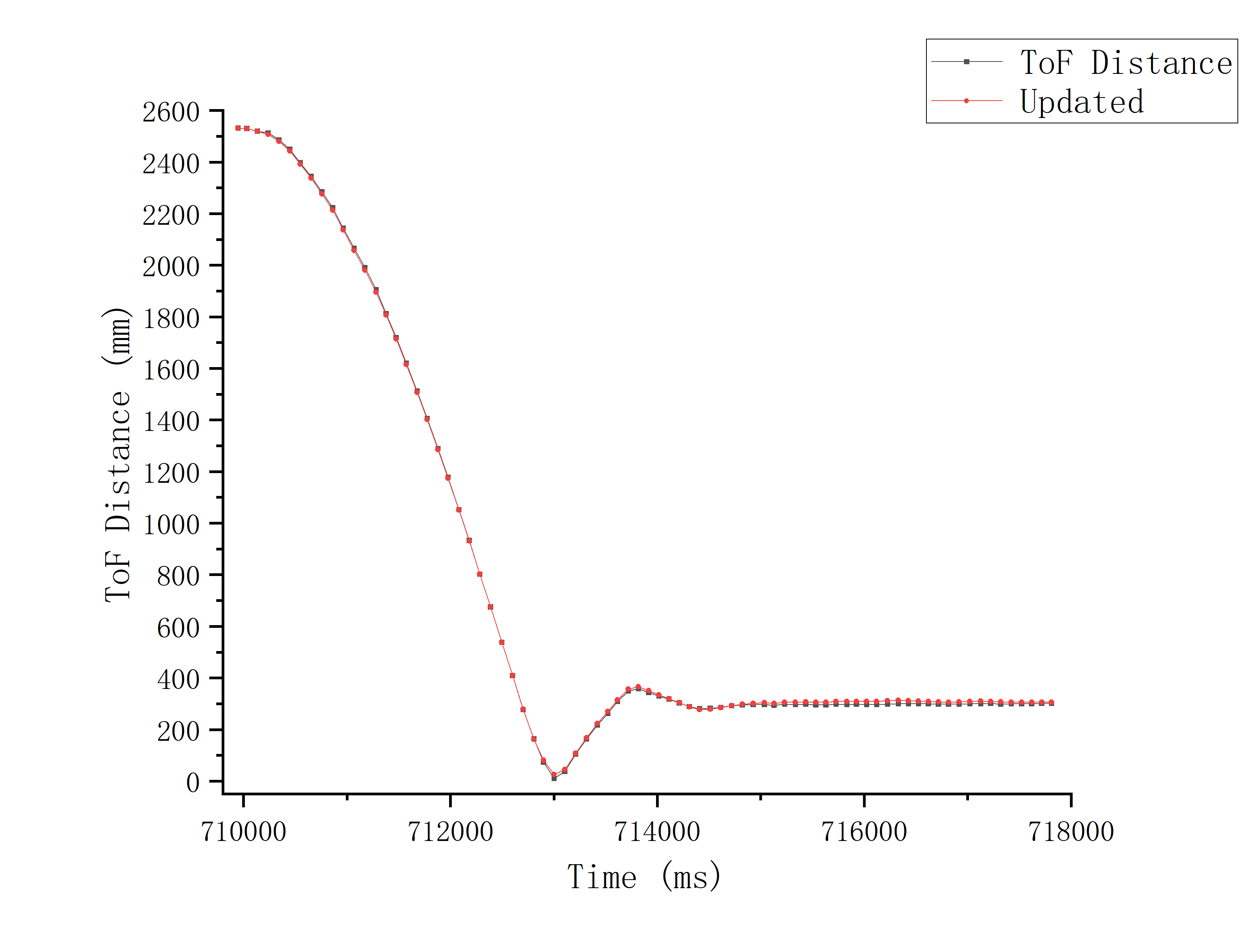
Having update, the simulation of Kalman Filter is highly coincident with the measured value by ToF, and the fit is perfect.

Kalman Filter Implementation

I implemente the full version Kalman Filter (including Prediction and Update) on the Artemis Board:

//prediction:
        sigma_1 = 10 * 10 / Delta_t;
        sigma_2 = 10 * 10 / Delta_t;
        sig_u = {sigma_1, 0,
                    0, sigma_2};
        A_d = {1, 1,
                0, 1-kf_d/kf_m*Delta_t};
        B_d = {0,
                Delta_t/kf_m};
        mu_p = A_d * mu + B_d * u;
        sigma_p = A_d * sigma * ~A_d + sig_u;
                
        get_tof();

//update:
        KF_cur = C * sigma_p * ~C + sig_z;
        KF_curr = 1/KF_cur(0,0);
        KF_cur = {KF_curr};
        KF_gain = sigma_p * ~C * KF_cur;
        y = {(float)dis};
        y_m = y - C * mu_p;
        mu = mu_p + KF_gain * y_m;
        sigma = (I_2 - KF_gain * C) * sigma_p;

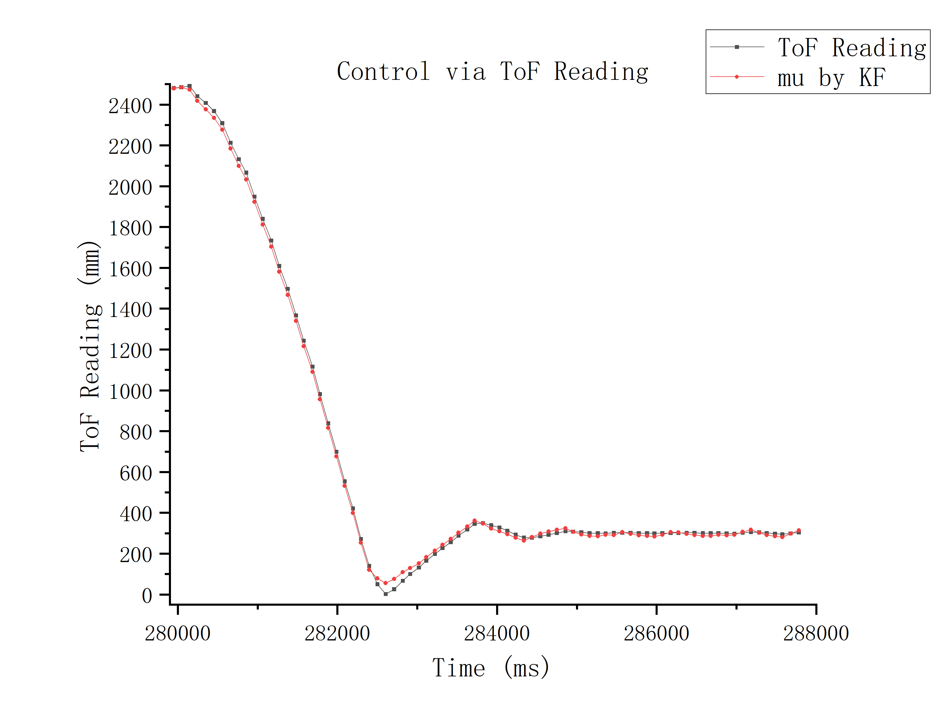
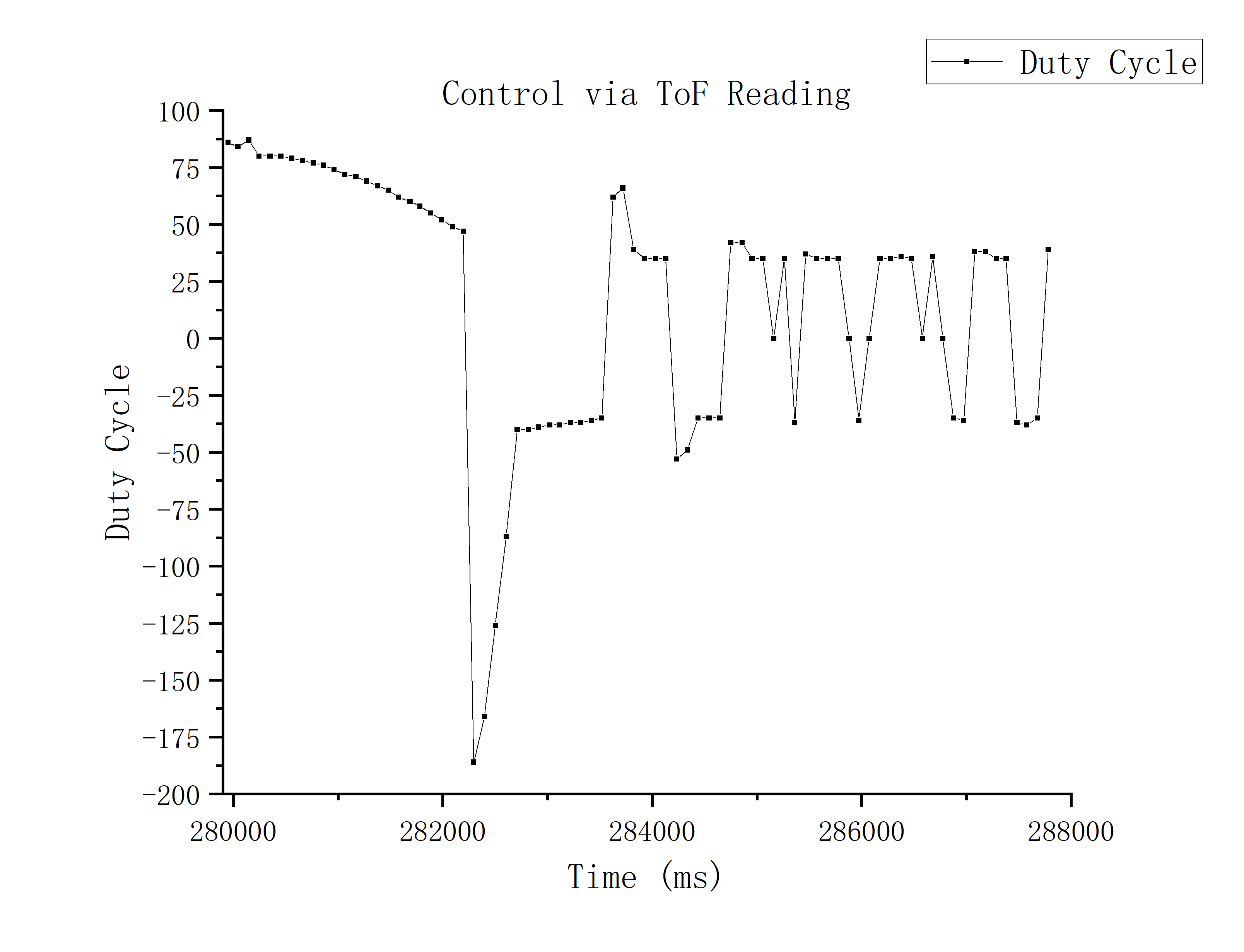
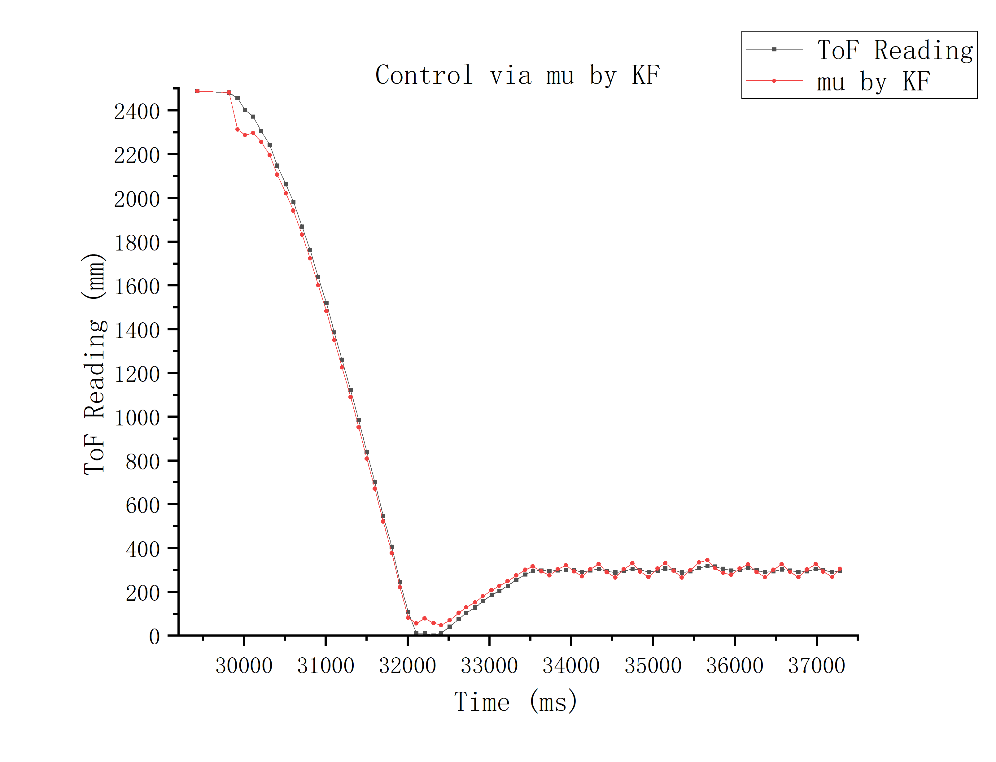
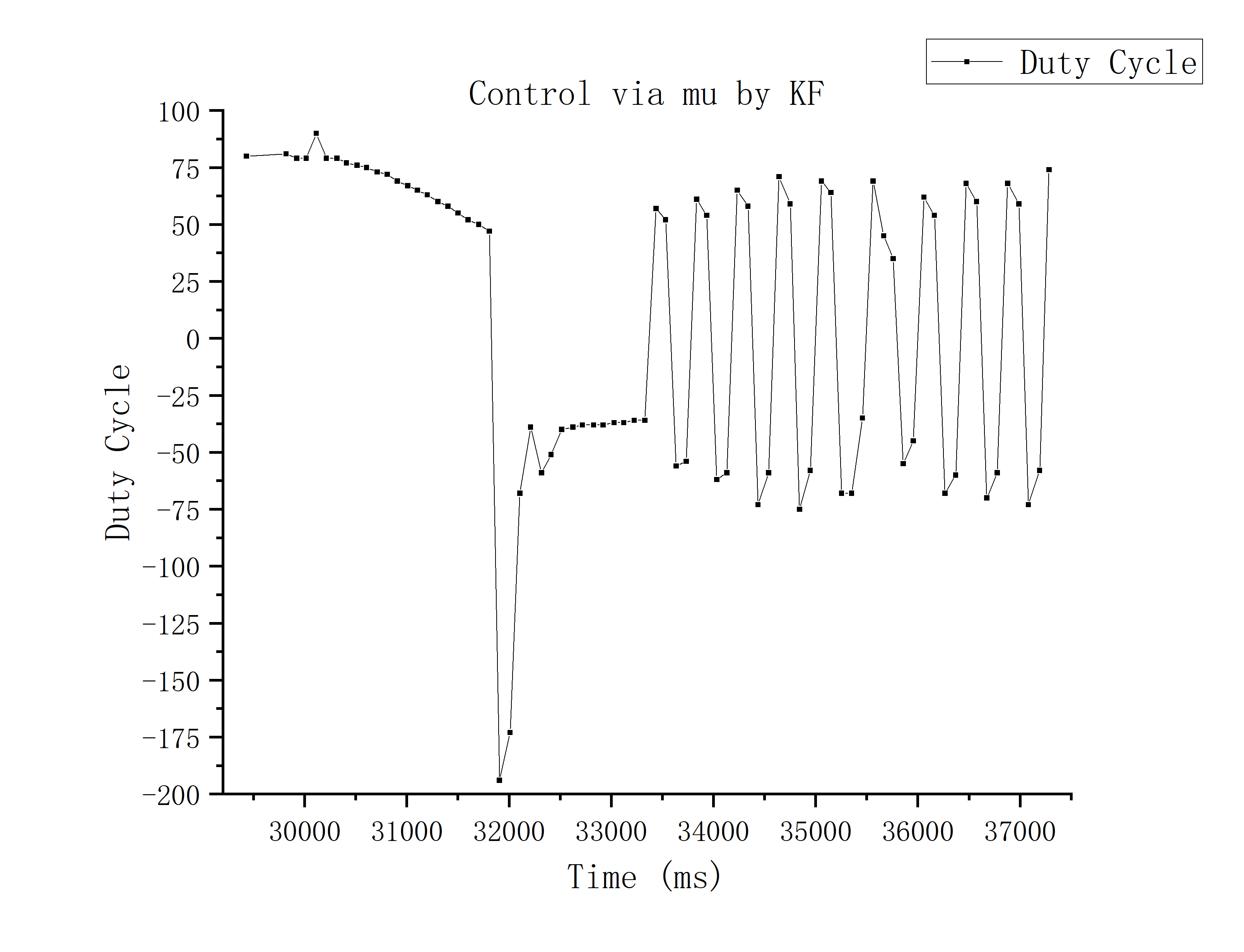
I compare the two situations running the car while calculating error via TOF readings or using mu generated by the Kalman Filter under the same PID settings:
K_p = 0.02; K_i = 0.003; K_d = 0.1; Deadband = 35; Set_point = 300;

Below is the demo video of implementation of Kalman Filter:

From the graphs and video above, we can see that the two methods have almost the same trend and speed approaching the set_point. However, when the car arrives near the set_point, in the subsequent fine-tuning process, the control via ToF readings is obviously more stable (see LAB 6).
This is because the value calculated by Kalman Filter fluctuates a little greater than ToF readings, which makes the value of the differential term in the PID control relatively larger, resulting in stronger negative feedback, which makes the car move back and forth wildly around the set_point. I will consider lowering the factor K_d for Differential and value of simga_3 (sensor's setting error), making the system trust the sensor more to reduce calculation fluctuation in the future.