Bayes Filter

The purpose of this lab is to implement grid localization using Bayes filter, which has two main step:
Prediction: Calculates the probability of the car at each position via odometry data
Update: Get observation data by executing a 360 degree rotation motion to update and determine the position of the car

Before executing Bayes filter, we need to complete some sub-functions first:

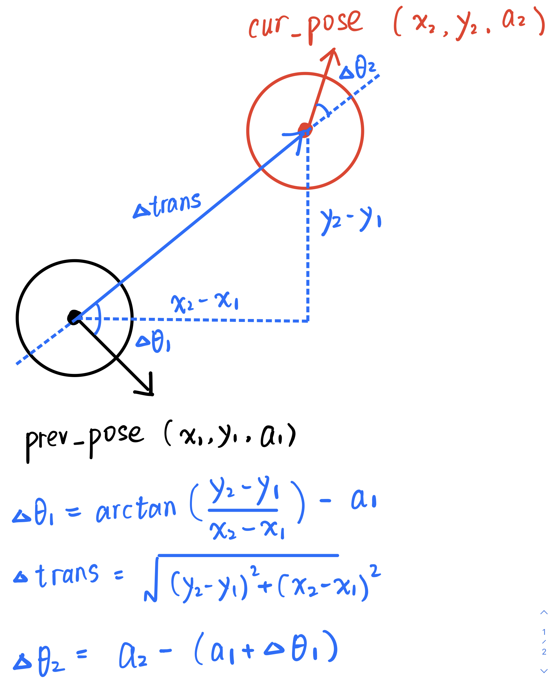
This function is used to calculate the angle of the two rotations and the distance of the translation given the prev_pose and the cur_pose.
According to the geometric relationship and formula shown in the figure below, we can easily complete this part.

    delta_rot_1 = (math.atan2(cur_pose[1]-prev_pose[1],cur_pose[0]-prev_pose[0]) - prev_pose[2])*180/np.pi
    
    delta_trans = math.sqrt((cur_pose[1]-prev_pose[1])**2+(cur_pose[0]-prev_pose[0])**2)
        
    delta_rot_2 = cur_pose[2]-(prev_pose[2]+delta_rot_1)

This function is used to calculate the probability of transitioning from previous state prev_pose to current state cur_pose given the control information actual_u using the formula shown below:

    u_bar = compute_control(cur_pose, prev_pose)
    
    p1 = loc.gaussian(mapper.normalize_angle(u[0]-u_bar[0]),0,loc.odom_rot_sigma)
    p2 = loc.gaussian(u[1]-u_bar[1],0,loc.odom_trans_sigma)
    p3 = loc.gaussian(mapper.normalize_angle(u[2]-u_bar[2]),0,loc.odom_rot_sigma)
    
    prob = p1 * p2 * p3

I did the normalization for the angle in this part and set the x of the Gaussian function to be (u - u_bar) while setting mu to 0.
This is because even if I can normalize the angles in compute_control, the two rotation data may still cause the angle to exceed the threshold [-180,180) in the Gaussian function.
For example: delta_rot1 = -170, delta_rot2 = 170;
Result of my approach: Gaussian(20, 0, sigma)
Result of Gaussian(u, u_bar, sigma): Gaussian(-340, 0, sigma)

This function is used to calculate belief for all possible current state x_t given the the control information actual_u and belief of all possible previous state x_t-1 using the formula shown below:

There are 12 x 9 x 18 = 1944 states in total, so in theory we need two big loops, one for the 1944 current states, the other for the 1944 previous states.
But when we compute the belief of a current state x_t, we can ignore the contribution from previous state x_t-1 whose belief is less than 0.0001.
Therefore, when I design the loop, I set the loop for previous states as the outer layer, and judge whether bel(x_t-1) is greater than 0.0001 before entering the inner loop for current states, otherwise it will not enter the inner loop, which saves a lot of computation resources.
In addition, I also calculate and store the central coordinates (x,y,a) in continuous world of all grid cell index (cx,cy,ca) in advance to reduce double-computation.

    #preprocess
    pose = np.zeros((mapper.MAX_CELLS_X,mapper.MAX_CELLS_Y,mapper.MAX_CELLS_A,3))
    for x in range(mapper.MAX_CELLS_X):
        for y in range(mapper.MAX_CELLS_Y):
            for a in range(mapper.MAX_CELLS_A):
                pose[x][y][a] = mapper.from_map(x, y, a)
    
    #initialization
    loc.bel_bar = np.zeros((mapper.MAX_CELLS_X,mapper.MAX_CELLS_Y,mapper.MAX_CELLS_A))
    #get actual_u
    actual_u = compute_control(cur_odom, prev_odom)
    #compute bel_bar
    #outer loop for previous states
    for x_prev in range(mapper.MAX_CELLS_X):
        for y_prev in range(mapper.MAX_CELLS_Y):
            for a_prev in range(mapper.MAX_CELLS_A):
                #check if bel > 0.0001
                if loc.bel[x_prev, y_prev, a_prev]> 0.0001:
                    #inner loop for current states
                    for x_cur in range(mapper.MAX_CELLS_X):
                        for y_cur in range(mapper.MAX_CELLS_Y):
                            for a_cur in range(mapper.MAX_CELLS_A):
                                loc.bel_bar[x_cur, y_cur, a_cur] += odom_motion_model(pose[x_cur][y_cur][a_cur], pose[x_prev][y_prev][a_prev], actual_u) * loc.bel[x_prev, y_prev, a_prev]

Finally, since we ignore the contribution of part of the previous states, the sum of the probabilities of bel_bar will be less than 1, so it needs to be normalized after the calculation.

This function is used to calculate likelihood of the 18 measurements given a state after a 360 degree rotation behavior using the formula shown below.
I set the current measurement data got by the rotation behavior loc.obs_range_data to be x in the Gaussian function, and the precached true measurements mapper.get_views to be mu.

    prob_array = 1
    for i in range(mapper.OBS_PER_CELL):
        prob_array *= loc.gaussian(loc.obs_range_data[i][0], obs[i], loc.sensor_sigma)

This function is used to update the data of bel for all current states x_t by combining the bel_bar and the probability calculated by sensor_model using the formula shown below:
Then normalize it after the computation is over so that the probabilities sum to 1.

    for x in range(mapper.MAX_CELLS_X):
        for y in range(mapper.MAX_CELLS_Y):
            for a in range(mapper.MAX_CELLS_A):
                loc.bel[x,y,a] = sensor_model(mapper.get_views(x,y,a)) * loc.bel_bar[x,y,a]
    
    loc.bel /= np.sum(loc.bel)

Implementation

Below are the demo videos of implementation:

In this video, even if the odometry line (red) deviates significantly from ground truth (green), the belief line (blue) calculated by Bayes filter is very close to ground truth, which shows that Bayes filter works well in general.

In this video, the 2-d grid space shows the value of bel_bar that is calculated by prediction_step. The lighter the grid, the greater the probability.
From the video we can find that the grid with higher probability displayed by the prediction is mostly close to the value of ground truth, which shows that Bayes filter does not only rely on the update_step, but the prediction_step also helps its work well.

Discussion

Having tested for multiple times, it is found that when the noise of the odometry value is too large, the accuracy of the prediction_step will be greatly reduced, but after the update_step, the value of belief can still be relatively close to ground truth.